Linear Regression

Linear regression attempts to model the relationship between two variables by fitting a linear equation to observed data. One variable is considered to be an explanatory variable, and the other is considered to be a dependent variable. For example, a modeler might want to relate the weights of individuals to their heights using a linear regression model. Before attempting to fit a linear model to observed data, a modeler should first determine whether or not there is a relationship between the variables of interest. This does not necessarily imply that one variable causes the other (for example, higher SAT scores do not cause higher college grades), but that there is some significant association between the two variables. A scatterplot can be a helpful tool in determining the strength of the relationship between two variables. If there appears to be no association between the proposed explanatory and dependent variables (i.e., the scatterplot does not indicate any increasing or decreasing trends), then fitting a linear regression model to the data probably will not provide a useful model. A valuable numerical measure of association between two variables is the correlation coefficient, which is a value between -1 and 1 indicating the strength of the association of the observed data for the two variables.
A linear regression line has an equation of the form Y = a + bX, where X is the explanatory variable and Y is the dependent variable. The slope of the line is b, and a is the intercept (the value of y when x = 0).

Least-Squares Regression

The most common method for fitting a regression line is the method of least-squares. This method calculates the best-fitting line for the observed data by minimizing the sum of the squares of the vertical deviations from each data point to the line (if a point lies on the fitted line exactly, then its vertical deviation is 0). Because the deviations are first squared, then summed, there are no cancellations between positive and negative values.

Example

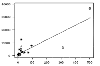
The dataset "Televisions, Physicians, and Life Expectancy" contains, among other variables, the number of people per television set and the number of people per physician for 40 countries. Since both variables probably reflect the level of wealth in each country, it is reasonable to assume that there is some positive association between them. After removing 8 countries with missing values from the dataset, the remaining 32 countries have a correlation coefficient of 0.852 for number of people per television set and number of people per physician. The r² value is 0.726 (the square of the correlation coefficient), indicating that 72.6% of the variation in one variable may be explained by the other. (Note: see correlation for more detail.) Suppose we choose to consider number of people per television set as the explanatory variable, and number of people per physician as the dependent variable. Using the MINITAB "REGRESS" command gives the following results:

The regression equation is People.Phys. = 1019 + 56.2 People.Tel.

To view the fit of the model to the observed data, one may plot the computed regression line over the actual data points to evaluate the results. For this example, the plot appears to the right, with number of individuals per television set (the explanatory variable) on the x-axis and number of individuals per physician (the dependent variable) on the y-axis. While most of the data points are clustered towards the lower left corner of the plot (indicating relatively few individuals per television set and per physician), there are a few points which lie far away from the main cluster of the data. These points are known as outliers, and depending on their location may have a major impact on the regression line (see below).

Data source: The World Almanac and Book of Facts 1993 (1993), New York: Pharos Books. Dataset available through the JSE Dataset Archive.

---

Outliers and Influential Observations

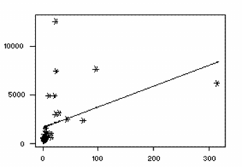
After a regression line has been computed for a group of data, a point which lies far from the line (and thus has a large residual value) is known as an outlier. Such points may represent erroneous data, or may indicate a poorly fitting regression line. If a point lies far from the other data in the horizontal direction, it is known as an influential observation. The reason for this distinction is that these points have may have a significant impact on the slope of the regression line. Notice, in the above example, the effect of removing the observation in the upper right corner of the plot: With this influential observation removed, the regression equation is now

 People.Phys = 1650 + 21.3 People.Tel. 

The correlation between the two variables has dropped to 0.427, which reduces the r² value to 0.182. With this influential observation removed, less that 20% of the variation in number of people per physician may be explained by the number of people per television. Influential observations are also visible in the new model, and their impact should also be investigated.

Residuals

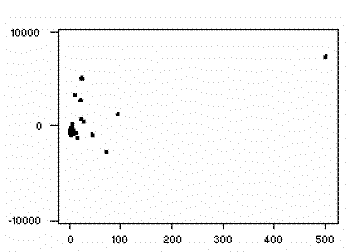
Once a regression model has been fit to a group of data, examination of the residuals (the deviations from the fitted line to the observed values) allows the modeler to investigate the validity of his or her assumption that a linear relationship exists. Plotting the residuals on the y-axis against the explanatory variable on the x-axis reveals any possible non-linear relationship among the variables, or might alert the modeler to investigate lurking variables. In our example, the residual plot amplifies the presence of outliers.

---

Lurking Variables

If non-linear trends are visible in the relationship between an explanatory and dependent variable, there may be other influential variables to consider. A lurking variable exists when the relationship between two variables is significantly affected by the presence of a third variable which has not been included in the modeling effort. Since such a variable might be a factor of time (for example, the effect of political or economic cycles), a time series plot of the data is often a useful tool in identifying the presence of lurking variables.

---

Extrapolation

Whenever a linear regression model is fit to a group of data, the range of the data should be carefully observed. Attempting to use a regression equation to predict values outside of this range is often inappropriate, and may yield incredible answers. This practice is known as extrapolation. Consider, for example, a linear model which relates weight gain to age for young children. Applying such a model to adults, or even teenagers, would be absurd, since the relationship between age and weight gain is not consistent for all age groups.